FastFlood Model Core
The Fastflood Model is a web-based simulation platform (www.fastflood.org), that combines industry-standard methodologies developed in the LISEM model since 1993 (Bout & Jetten, 2018), with recent innovations in flood modelling (Bout et al., 2023). It features Interactive speed, easy-to-use model setup and simulation, and the accuracy of industry-standard methods. The method is based on the steady-state assumption, which enables high computational efficiency. However, steady-state situations are exceptional in nature. For this reason, the model uses a series of algorithms to compensate and correct the derived flow heights while avoiding the need for dynamic simulations.
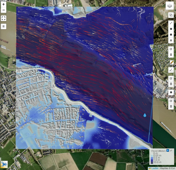
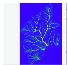
FastFlood detailed simulation results using bathymetry and topography data in the Rhine river, Netherlands.
The Fastflood model and methodology was introduced by Bout et al. (2023). In this paragraph a short overview of the model setup is given. The model contains 5 key steps, with critical underlying assumptions. The steps are as follows;
- Terrain correction
Using a Fast Sweeping Algorithm, gridcells in the elevation model are forced to be at least the elevation of the lowest neighbor, with some additional small value. The resulting elevation model is monotonically increasing.
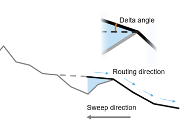
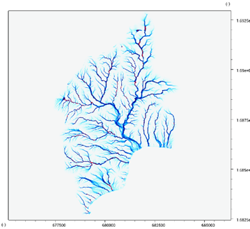
- Flow network derivation
The monotonically increasing elevation model can be used to create a flow network by taking the local derivatives of the elevation and using the angle of steepest descent as a flow direction. Optionally, these angles might be limited to 4 or 8 directions to mimic a D4 or D8 flow direction network.
- Steady-state discharge routing
Over this network, a steady-state discharge is routed through a simple flow accumulation, with another speed up by using fast sweeping numerical algorithms.
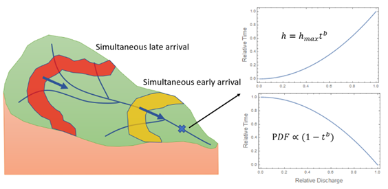
- Partial steady-state correction
Natural events rarely reach a steady-state flow.
Based on catchment properties and event
duration, a correction is applied to estimate
Actual peak flow.
- Flow depth reconstruction
Finally, peak flow rates are used to reconstruct a spatial
peak flow depth field (flood map). This step used an inversion of Mannings equations for a rectangular channel. In this research, a revision on this inversion is introduced with significant improvements.
The key assumptions which are taken in the methodology relate to the non-dynamic nature of the algorithms. Only peak discharges, flow depths and velocities are estimated. As a result, input of precipitation is required in a duration-intensity pair, and cannot be a full rainfall graph. The steady-state assumption used in step 3 is corrected in step 4, but the correction step relies on various assumptions about catchment homogeneity. For more details on the derivation of this correction see Bout et al., (2023).